The curse of dimensionality
The curse of dimensionality arises from the fact that at higher dimensions, the features space becomes increasingly sparse for a fixed-size training set. Because of this, many machine learning algorithms that work fine in low dimensional features space have their performance degraded severely in the features space in higher dimensions. Due to the sparsity, the entire training set only occupies a microscopic fraction of the features space. This sparsity can degrade the performance of machine learning algorithms because they rely on the availability of a dense data space to learn patterns effectively.
To quote Prof. Pedro Domingos of University of Washington in his excellent article: A Few Useful Things to Know About Machine Learning:
Even with a moderate features dimension of 100 and a huge training set of a trillion examples, the latter covers only a fraction of about $10^{-18}$ of the input space.
Let’s try to understand this a bit more with a few simple mathematical intuitions:
Intuition 1: Consider a pizza with a rather odd slice which cuts it in two concentric circles. Let’s also assume that the size of the pizza is significantly larger than the typical large size pizza. For the sake of assigning some numbers, let’s say that its radius is 1’ whereas the the slice has a radius of 1/2’.
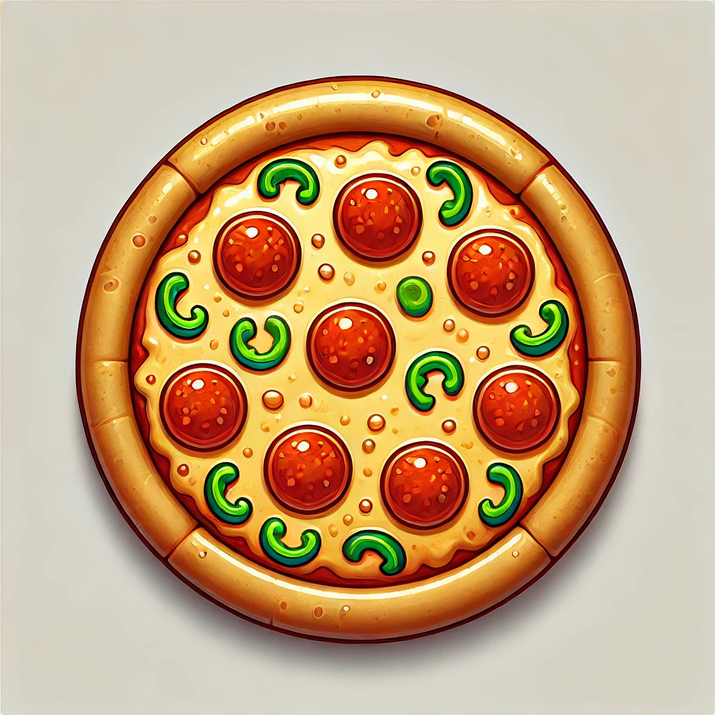
Let’s calculate how much area is sliced out by the smaller circle: \(A = \pi * r^{2}\)
\[\implies A_{large} = \pi * 1 * 1 = \pi \quad sq.ft\] \[A_{small} = \pi * \frac{1}{2} * \frac{1}{2} = \frac{\pi}{4} \quad sq.ft\]Remaining area = $A_{large} - A_{small} = \frac{3\pi}{4} \quad sq.ft$ .
This means only 25% area is sliced out by the smaller pizza whereas 75% of the crust is still present in the remaining pizza.
Let’s extrapolate this example to 3 dimensions to a sphere of a unit radius. If a smaller sphere of radius one-half is carved out. We can compute the volume remaining in the sphere in a way similar to the pizza example:
Remaining volume = $V_{large} - V_{small} = \frac{4}{3} * \pi * 1^{3} - \frac{4}{3} * \pi * (\frac{1}{2})^{3} = \frac{4}{3} * \pi * \frac{7}{8}$
We can see that only 12.5% volume of the sphere is carved out and 87.5% of the volume is still there.
This can be generalized to higher dimensions – as we increase the dimensionality, the volume of a hypersphere is concentrated more and more in its outer skin. If a fixed-size training set is uniformly distributed in an $n$-dimensional hypersphere, most of them will be closer to the edge of the hypersphere and far apart from each other.
Intuition 2: Consider six points lying on the circumference of a circle of unit radius such that they are equidistant from each other. By simple geometry, you can find that the angle between any two adjacent points is 60 degrees.
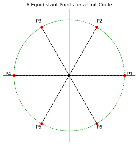
However, if those same 6 points located on the outer surface of a unit sphere, the angle between the adjacent point increases from 60 degrees to 90 degrees.
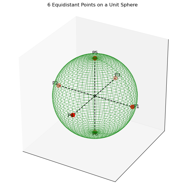
This can be extrapolated to higher dimensions and can be inducted that the angle between adjacent points will keep on increasing.
From Prof. Pedro – Higher dimensions break down our intuitions because they are very difficult to understand. Naively, one might think that gathering more features never hurts, since at worst they provide no new information about the class. But in fact their benefits may be outweighed by the curse of dimensionality.
A word of caution: Although distance as a metric works well in the above intuition qualitatively, and is traditionally used in $k$ dimensions ($k \le 3$), it should be avoided in the feature spaces with higher values of $k$ ($k \gt 3$). Because of this, algorithms which use L1 or L2 norms like K-nearest neighbors become ill-defined in higher dimensions. The article by Aggarwal et al., “On the Surprising Behavior of Distance Metrics in Higher Dimensional Space” discusses this in great detail.
Distance is an ill-defined metric in higher dimensions
The distribution of distances from the origin in various dimensions follows specific patterns. Here’s a summary for a random point uniformly distributed inside a unit hypercube or hypersphere. For general $n$ dimensions, the distance ( r ) from the origin follows a chi distribution with ( n ) dimensions. The probability density function (PDF) is given by –
\[f(r) = \frac{r^{n-1} e^{-r^2/2}}{2^{n/2-1} \Gamma(n/2)}\]for $r \geq 0$, where $\Gamma$ is the gamma function.
The chi distribution generalizes to various dimensions, with the shape and scale influenced by the number of dimensions. In high dimensions, distances tend to cluster around a certain value, leading to a more concentrated distribution.
K-Nearest Neighbors
KNN is a simple, non-parametric algorithm used for classification and regression. The basic idea is to classify a data point based on the majority class of its nearest neighbors in the feature space. However, KNN relies heavily on the concept of distance, typically using Euclidean distance, which becomes less reliable as dimensionality increases.
How KNN Works
-
Compute Distance: For a given test point, calculate the distance between this point and all points in the training dataset.
-
Sort Neighbors: Sort the training points in ascending order of distance.
-
Assign Class: Assign the class of the majority of the k closest points (for classification) or compute the average of the k closest points (for regression).
Struggles of K-Nearest Neighbors in higher dimensions
-
Distance Metrics Become Less Effective: In high-dimensional spaces, the concept of “distance” can become less intuitive because the distances between all pairs of points tend to be similar. The following plot for the ratio of the maximum pairwise distance to the minimum pairwise distance shows that in higher dimensional feature spaces, KNN may struggle because all points seem almost equidistant from each other, making it difficult to distinguish between neighbors effectively.
Moreover, as seen in the chi distribution for high dimensions, the distances between points become concentrated around a certain value. This means that, in high-dimensional spaces, the distance between any two points tends to be similar which typically results in distance-based metrics losing their effectiveness in high-dimensional spaces. This can lead to less meaningful neighbor-based classifications or regressions.
-
Increased Computational Cost: The need to calculate the distance between the test point and all training points for every prediction becomes computationally expensive as dimensionality increases.
-
Overfitting: In high-dimensional space, the model might overfit to the noise in the data rather than capturing the underlying patterns.
Dealing with the Curse of Dimensionality
-
Dimensionality Reduction: Techniques like Principal Component Analysis (PCA) or t-SNE reduce the number of dimensions while preserving as much variance as possible
-
Feature Selection: Identify and select the most relevant features, ignoring those that contribute little to the model’s performance.
-
Regularization: Apply regularization techniques to prevent overfitting by penalizing overly complex models.
-
Alternative Distance Metrics: Instead of Euclidean distance, use other metrics like Manhattan distance or Mahalanobis distance that might work better in high dimensions.
Dimensionality reduction
Dimensionality reduction aims at simplifying large datasets by reducing the number of input variables while preserving as much information as possible. It also enhances interpretability, reduces noise, and improves the efficiency of algorithms.
Principal Component Analysis
It’s a tool for providing a low-dimensional representation of the dataset without losing much of the information. By information we meant, it tries to capture as much variation in the data as possible.
The new features can be projected in a much smaller space whose axes are called principal components. These axes are orthogonal to each other and their direction can be interpreted as the direction of maximum variance. The orthogonality between the principal components ensures no correlation between each other.
PCA is very sensitive to the data scaling. Features with larger scales or variances will completely dominate the PCA results. PCA directions will be biased towards these features, which will potentially lead to the incorrect representations of the structure of the data. It is therefore highly recommended to standardize the data first before applying it.
Linear Discriminant Analysis (LDA)
This is another technique used primarily in classification tasks. Unlike PCA, which is unsupervised, LDA is a supervised method that seeks to maximize the separation between multiple classes by projecting the data onto a lower-dimensional space. This makes LDA particularly useful when the goal is not only to reduce dimensionality but also to enhance the discriminative ability of the model by highlighting differences between classes.
Both PCA and LDA are linear algorithms – the dimensionality reduction mapping is linear. In PCA, it’s the matrix of eignevectors of the covariance matrix:
\[x' = V^{T} x\]In addition to these, there are also non-linear methods like t-SNE, umap, and autoencoders which can also provide more compact representation on the data.
Benchmarks
To illustrate the concept, I’ll talk about the performance of the KNN algorithm with and without PCA. To analyze it further, I’ll compare the results with one more supervised learning algorithm with and without PCA.
The dataset consists of 10000 samples containing four classification labels. The dataset is highly imbalanced and the class pareto looks something like:
K-Nearest Neighbors without PCA
Without PCA, we can see that the model performance saturates at about 500 features. Furthermore, while creating the synthetic dataset, I kept the number of informative features to be:
\[\mathrm{num\_informative\_features} = \begin{cases} \mathrm{num\_features}, & \mathrm{num\_features} <= 50 \\ 50, & \mathrm{num\_features} > 50 \end{cases}\]From the plot below, we can see that adding more features after 500 did not have much impact on model’s performance:
However, we can see the model’s performance is terrible on the minority class. It maxed out at a feature dimension of 10 and then took a big dip in the F1-score. This is true for all the classes, their F1-score maxed out at around 10-100 and then degraded for increasing number of features. This is because for a given number of features, we don’t have enough data. This results in the feature space being increasingly sparse as mentioned earlier. Algorithms based on the Euclidean distance as the metric would struggle.
K-Nearest Neighbors with PCA
Including PCA didn’t yield any meaningful improvements – individual class performance is still maxed out at about 10-50 features. This is in the ballpark of the num_informative_features defined above. This means our entire feature space can be compressed to 50 dimensions without losing much information. This is indeed what I get from calculating the number of features with explained_variance_ratio_ $ > 0$:
Histogram-Based Gradient Boosting
According to the Scikit-learn documentation, Histogram-Based Gradient Boosting (HGBT) models may be one of the most useful supervised learning models in scikit-learn. They are based on a modern gradient boosting implementation comparable to LightGBM and XGBoost.
As such, HGBT models are more feature rich than and often outperform alternative models like random forests, especially when the number of samples is larger than some ten thousands. Not to mention, it is much faster than algorithms like random forests. Keeping all the characterisitics of our dataset same as the KNN, let’s see how Histogram gradient boosting classifier performed on it:
Even with this algorithm, we can see the model’s performance on the validation set with 5000 features is similar to the one with 50 features for most of the classes. Increasing the number of features by 100x did slow down the training even if the gains were minimal. Although the model’s performance on the minority class did improve by adding more features, it is still less than what it was at 10 features.
HGBT with PCA
What would happen if we hook up PCA with the histogram gradient boosting? Well, the overall trend for the classwise performance stayed the same but something interesting happened with the classwise F1-scores – they all improved by adding dimensionality reduction. The minority class got a significant 12% improvement!! The maximum happened at num_features of 200. These features were compressed by the PCA before feeding them to the HistogramGradientBoosting classifier which outperformed all the previous cases by significant margin:
Final Thoughts
The curse of dimensionality is a significant challenge in machine learning, particularly for algorithms like K-Nearest Neighbors that rely on distance measurements. As dimensionality increases, the performance of such algorithms tends to degrade due to the sparsity of data and the loss of meaningful distance metrics.
However, techniques like dimensionality reduction, feature selection, better algorithms, and the use of alternative distance metrics can help mitigate these issues. Understanding the curse of dimensionality and its effects is crucial for building effective machine learning models, especially when dealing with high-dimensional datasets.
References
- https://stats.stackexchange.com/questions/451027/mathematical-demonstration-of-the-distance-concentration-in-high-dimensions
- https://homes.cs.washington.edu/%7Epedrod/papers/cacm12.pdf
- https://mathoverflow.net/questions/128786/history-of-the-high-dimensional-volume-paradox/128881#128881
- https://stats.stackexchange.com/questions/99171/why-is-euclidean-distance-not-a-good-metric-in-high-dimensions