Mathematical details behind self-attention
Introduction
In the ever-evolving landscape of artificial intelligence and machine learning, the self-attention mechanism has emerged as a pivotal innovation, revolutionizing the way models understand and process information. Introduced as part of the transformer architecture, self-attention has rapidly become a cornerstone in natural language processing (NLP) and beyond.
At its core, the self-attention mechanism allows a model to weigh the importance of different words in a sentence when making predictions. Unlike traditional sequence processing methods, such as recurrent neural networks (RNNs) and long short-term memory networks (LSTMs), which process data sequentially, self-attention enables models to consider the entire sequence of words simultaneously. This parallelism not only speeds up training and inference but also provides a more nuanced understanding of the relationships between words, capturing dependencies regardless of their distance from each other in the text.
The intuitive appeal of self-attention lies in its ability to dynamically adjust the focus of the model based on the context. For instance, in the sentence “The cat sat on the mat because it was tired,” the word “it” refers to “the cat.” A self-attention mechanism can learn this relationship by assigning higher importance to “the cat” when processing “it,” enhancing the model’s comprehension of pronoun references and improving overall performance on tasks such as translation, summarization, and question answering.
Moreover, self-attention is not limited to NLP. Its versatility extends to other domains like computer vision, where it helps in tasks such as image classification and object detection by allowing models to focus on relevant parts of an image.
We will try to understand how exactly self-attention works and the intuitions behind it in more detail in this post. Although there already exists tons of great resources on self-attention mechanism, in order to understand it better for my learnings, I wanted to get some visual intuition behind this concept. One other motivation to write this post is to see how beautifully it leverages the concepts of linear-algebra. After explaining it conceptually, I will end this post by implementing multihead self-attention using just vanilla PyTorch.
Embeddings
Embeddings represent words/tokens as high dimensional vectors in a way that similar words are located closed to each other. Words having high similarity are placed closer to each other whereas words with low similarity will be pushed far away from each other in this space.
How are the words placed together or far apart?
Similar words are placed together by the context, meaning the words in the sentence decide how much closer two words will be placed to each other.
How do we find the similarity between two words though? Well, it turns out we first need to represent the words/tokens as vectors in the embedding space and use a measure of similarity between those two vectors. There are multiple choices available for such a metric.
Word Similarity
- Although it seems convenient but euclidean distance is not the correct measure of the word similarity
- Measures of the word similarity in the embedding space:
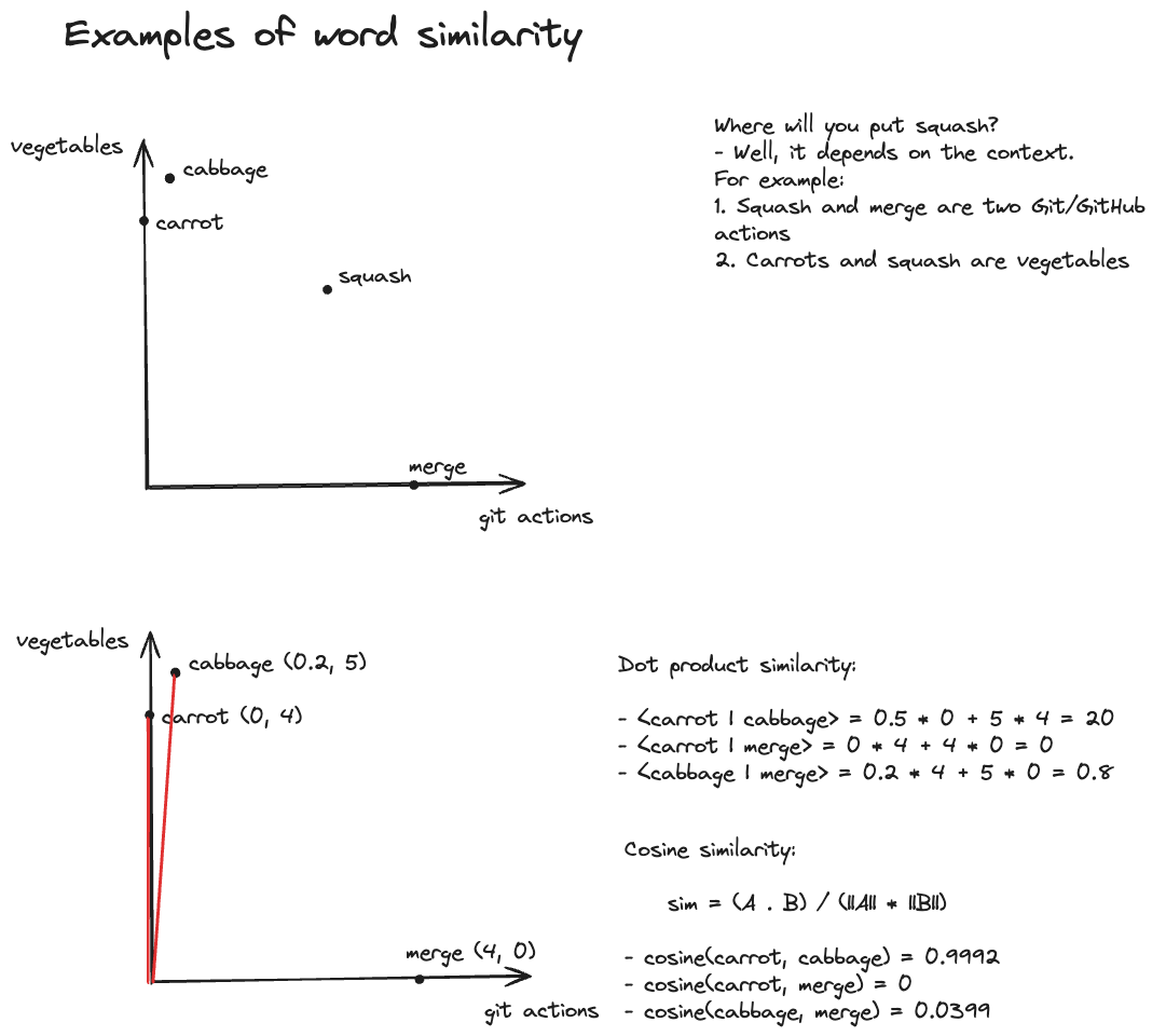
- Dot product: Elementwise product followed by the sum of the two words being represented as vectors:\(u = \sum_{i=0}^{n} a_{i} \cdot b_{i}\)
- Cosine similarity: Similar to dot product but this method measures the similarity between two words by computing the cosine of the angle ($\theta$) between two words when being represented as vectors in the embedding space. Dot product becomes the cosine similarity when the norm of the vectors is unity: \(u = \cos(\theta)\)
- Scaled dot product (used in self-attention): This is just the dot product divided by the square root of the length of the vectors. The division is done to scale the length when the dimensionality of the embedding space is too high to prevent the blowing-up of the values of the dot product
The top plot in the above image shows an example where are embedding space is only two dimensional with $y$-axis as vegetables and $x$-axis as various git actions. It demonstrates how the context is used in finding the similarities between words/tokens – it will place “squash” closer or farther to one axis based on the relationship between other words of the sentence.
The bottom plots assigns some coordinates to the points for interpretability and calculates dot product and cosine similarities.
So what is self-attention?
NOTE: This is my take on the self-attention, it is adapted from the excellent video by Luis Serrano. Please make sure to check it out for more details.
Now that we have talked about word similarity, we can play with linear transformations a bit more. For simplicity and for visualization, we will assume that our embeddings space is two dimensional.
Let’s take another example, consider the following two statements:
- A bat lives in the cave
- A tennis racket and a baseball bat
Without any context, it would be hard for the model to place the word “bat” in the embeddings space – it would probably be placed in the middle. Let’s make it more concrete and assign some coordinates to each one of the words (we ignore the grammatical tokens for now).
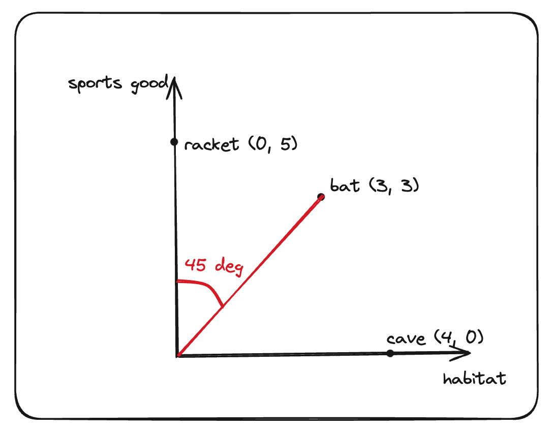
Like before, we can now compute the similarity between these words using the cosine similarity:
| Bat | Cave | Racket | |
|---|---|---|---|
| Bat | 1 | 0.71 | 0.71 |
| Cave | 0.71 | 1 | 0 |
| Racket | 0.71 | 0 | 1 |
From the above similarity table, we can see the individual contributions (as weights) from other words for a given word. In the language of linear algebra, we can write the individual words as a linear combination (weighted sum) of the other:
- A bat lives in the cave
Bat = 1 * Bat + 0.71 * Cave Cave = 0.71 * Bat + 1 * Cave - A tennis racket and a baseball bat
Bat = 1 * Bat + 0.71 * Racket
Racket = 0.71 * Bat + 1 * Racket
In machine learning applications, it’s convenient to normalize the coefficients so that they sum to 1. Normalization increases the interpretability of the coefficients as they can be assumed as the relative weights or the probabilities. This is typically done by applying softmax operation. Moreover, it also prevents the coefficients from blowing up and helps in maintaining the stability during training. After applying the softmax, the coefficients of the above linear transformations take the values:
Bat = 0.57 * Bat + 0.43 * Cave
Cave = 0.43 * Bat + 0.57 * Cave
Bat = 0.57 * Bat + 0.43 * Racket
Racket = 0.43 * Bat + 0.57 * Racket
With the help of some coordinate geometry, it is not hard to see that after adding contributions from the other words, we are basically moving each word in the embedding space.
In other words, after getting the “context” from other words in the first sentence, the first set of equations basically shifted the “Bat” and the “Cave” towards each other. The equations,
Bat = 0.57 * Bat + 0.43 * Cave
Cave = 0.43 * Bat + 0.57 * Cave
are the context vectors for the “Bat” and the “Cave” tokens in the embedding space.
On a higher level, this is exactly how the attention mechanism works – we took a word token (query) and look in its own sequence (keys) to find the information that should be used from other words to create a context vector.
To summarize, we took the following steps to calculate the context vector:
- Calculate attention scores: The attention mechanism calculates the similarity scores between each pair of the input sequence. Higher the similarity score, the more relevant is the key to the current query. I used cosine similarity but in the original “Attention is all you need” paper, it is done by calculating scaled dot-product similarity.
import numpy as np from numpy.linalg import norm # define coordinates of words racket = [0, 5] # x-coordinate: 0, y-coordinate: 5 bat = [3, 3] # x-coordinate: 3, y-coordinate: 3 cave = [4, 0] # x-coordinate: 4, y-coordinate: 0 # convert the list of coordinates to a NumPy array embed_vectors = np.array([bat, cave, racket]) # create a function for creating cosine similarity def cos_sim_matrix(vectors): # calculate the norms of each vector norms = norm(vectors, axis=1) # calculate the dot product between each pair of vectors dot_products = np.dot(vectors, vectors.T) # calculate the outer product of the norms norm_products = np.outer(norms, norms) # calculate the cosine similarity matrix cosine_similarity = dot_products / norm_products return np.round(cosine_similarity, 2) # find similarity similarity_matrix = cos_sim_matrix(embed_vectors) print(similarity_matrix) # prints # array([[1. , 0.71, 0.71], # [0.71, 1. , 0. ], # [0.71, 0. , 1. ]]) - Normalization (Softmax): Softmax function is applied on the attention scores to yield the probabilities. The softmax ensures the weights sum up to 1, which is helpful for training stability and interpretability.
# similarity scores for the first sentence bat_cave = similarity_matrix[:1, :2] # apply softmax to it bat_cave = np.exp(bat_cave) softmax = bat_cave / np.sum(bat_cave, axis=1) softmax = np.round(softmax, 2) print(softmax) # prints # array([[0.57, 0.43]]) - Weighted Summation: Lastly, attention weights are multiplied by the corresponding values and these weighted contributions are then summed up to create a context vector.
Queries, Keys and Values
In the previous section, while explaining the connection between self-attention and context vector, three terms were mentioned – query, key and value. These terms are actually borrowed from the domain of information retrieval and databases, where similar concepts are used to store, search, and retrieve information.
A “query” is analogous to a search query in a database. It represents the current item (e.g., a word or token in a sentence) the model focuses on or tries to understand. The query is used to probe the other parts of the input sequence to determine how much attention to pay to them.
The “key” is like a database key used for indexing and searching. In the attention mechanism, each item in the input sequence (e.g., each word in a sentence) has an associated key. These keys are used to match with the query.
The “value” in this context is similar to the value in a key-value pair in a database. It represents the actual content or representation of the input items. Once the model determines which keys (and thus which parts of the input) are most relevant to the query (the current focus item), it retrieves the corresponding values.
For self-attention, this is where the actual magic happens: instead of using the embedding vectors of the input tokens directly as key-query-value, we calculate key, query and value vectors during the training. These vectors are actually obtained by transforming the input embedding vectors with three matrices – K, Q and V. There is something special about these matrices which I will cover in the next section.
Intuition behind K, Q and V matrices
From the basic linear-algebra, we know that matrices are nothing but the linear transformations or rules that operate on vectors and change their properties like rotate them by a certain angle, reflect them about some axis, etc. These trainable matrices for query, keys and values do something similar – stretch, shear, or elongate the manifolds such that the similarity of the alike words increases whereas for dissimilar words it decreases. These matrices are adaptive to the dataset, meaning they are optimized during the course of training using backpropagation.
Let’s try to understand this by a few examples. Consider a set of two vectors whose $x$ and $y-$ coordinates are represented as column vectors:
\(\qquad\) \(v_{1}=\begin{pmatrix} 1 \\ 0 \end{pmatrix}\), \(v_{2}=\begin{pmatrix} 0 \\ 1 \end{pmatrix}\)
and let’s analyze the effect of the linear transformations on these vectors as well as their similarity. The original similarity between $v_{1}$ and $v_{2}$ is 0 since they are orthogonal to each other.
Example 1: Stretching in one direction
Consider a 2D matrix A:
\[A = \begin{pmatrix} 3 & 0 \\ 0 & 1 \end{pmatrix}\]This matrix stretches the vectors along $x$-axis by a factor of 3 while leaving the $y$-axis unchanged. The matrix $A$ transforms $v_{1}$ and $v_{2}$ as follows:
\[Av_{1} = \begin{pmatrix}3 & 0 \\ 0 & 1 \end{pmatrix} \begin{pmatrix}1 \\ 0 \end{pmatrix} = \begin{pmatrix}3 \\ 0 \end{pmatrix}\] \[Av_{2} = \begin{pmatrix}3 & 0 \\ 0 & 1 \end{pmatrix} \begin{pmatrix}0 \\ 1 \end{pmatrix} = \begin{pmatrix}0 \\ 1 \end{pmatrix}\]The similarity still stays at zero because the resultant vectors are still orthogonal to each other but with different norms.
Example 2: Effect on dissimilar vectors
For this case, let’s make things a bit more complicated and see how the matrix $A$ from example 1 above transforms two arbitrary vectors:
\(\qquad\) \(v_{3}=\begin{pmatrix}1 \\ 1 \end{pmatrix}\), \(v_{4}=\begin{pmatrix}-1 \\ 0 \end{pmatrix}\)
For the sake of comparison, I will calculate the similarity scores as well as attention weights of these:
# define the vectors as column arrays
v3 = np.array([[1], [1]])
v4 = np.array([[-1], [0]])

# matrix A
A = np.array([
	[3, 0],
	[0, 1]
])

# stack vectors v3 and v4 to create similarity
embed_vectors1 = np.array([
	v3.squeeze(),
	v4.squeeze()
])

similarity_matrix1 = cos_sim_matrix(embed_vectors1)
print(similarity_matrix1)
# prints
# array([[ 1. , -0.71],
#        [-0.71, 1. ]])

attn_weights1 = softmax(similarity_matrix1[0])
print(attn_weights1)
# prints
# array([0.85, 0.15])
Let’s see how vectors $v_{3}$ and $v_{4}$ attention weights change after transforming by matrix $A$:
# matrix multiplication
av3 = A @ v3
av4 = A @ v4

embed_vectors2 = np.array([
	av3.squeeze(),
	av4.squeeze()
])

similarity_matrix2 = cos_sim_matrix(embed_vectors2)
print(similarity_matrix2)
# prints
# array([[ 1. , -0.95],
#        [-0.95, 1. ]])

attn_weights2 = softmax(similarity_matrix2[0])
print(attn_weights2)
# prints
# array([0.88, 0.12])
From this simple exercise, we can see that transforming vectors with matrices can increase/decrease the similarity score and hence the attention weights between two vectors. This is what K, Q and V do to the input embedding vectors. They are trainable meaning during the course of training, their weights will be optimized to change the manifold. This will increase/decrease the similarity between tokens on the basis of the loss function optimization during training.
To put in simpler terms, consider a python dictionary where each key refers to the name of a user and the corresponding values contains the addresses and the phone numbers. Let’s say we need to find the details of the users with names similar to “Alex”. In this case, “Alex” is the query which is the search string. Keys will be all the user names in the dictionary (dictionary keys). But we don’t want to fetch the keys, rather we want the addresses and the phone numbers associated with the keys. Here, the addresses and the phone numbers are the values.
For this example, think of K, Q and V matrices as rules to standardize the user names and their corresponding keys – make them lowercase, remove the punctuations, etc.
Understanding these mathematical details allows us to appreciate this concept even more, not to mention it gives us an insight about its internal machinery. Now, I will move on to implementing self-attention using plain PyTorch. I should mention that much of this implementation code is resulted from my notes from a great read by Sebastian Raschka – Build a Large Language Model (From Scratch). Check it out if you want to understand the inner workings of the LLMs.
Implementing Multi-head self-attention
Multi-head self-attention applies self-attention multiple times at once, with each self-attention instance being called a head, each with different key, query, and value transformations of the same input, and then combines the outputs.
import torch
import torch.nn as nn

# Helper class for Self-Attention calculation
class SelfAttention(nn.Module):
	def __init__(self, input_dim, output_dim):
		super().__init__()
		self.output_dim = output_dim

		# matrices for Query, Key, and Value
		self.W_query = nn.Linear(
			in_features=input_dim, out_features=output_dim, bias=False
		)
		self.W_key = nn.Linear(
			in_features=input_dim, out_features=output_dim, bias=False
		)
		self.W_value = nn.Linear(
			in_features=input_dim, out_features=output_dim, bias=False
		)

	def forward(self, x): # x shape: (N, input_dim), N: number of tokens
		queries = self.W_query(x)
		keys = self.W_key(x)
		values = self.W_value(x)

		# attention scores
		attn_scores = queries @ keys.T # N x N

		# attention weights
		attn_weights = torch.softmax(attn_scores / self.d_out**0.5, dim=-1)

		# compute context vector
		context_vec = attn_weights @ values # N x output_dim

		return context_vec

# Multi-head self-attention
class MultiHeadAttention(nn.Module):
	def __init__(self, input_dim, output_dim, num_heads):
		super().__init__()
		self.heads = [
			SelfAttention(input_dim, output_dim)
			for _ in range(num_heads)
		]

	def forward(self, x):
		return torch.cat([head(x) for head in self.heads], dim=-1)
While the above implementation is pretty simple to understand for learning purposes, it is not meant for production. It is also not suitable for tasks where we want to mask the information of the future words and each word prediction only depends on the previous words. In such cases, we use something called as causal attention where we mask the information about the future words in the sequence thereby prohibiting the model’s access of them.
Moreover, the above implementation is not very computationally efficient – self-attention of all the heads is calculated sequentially with the for loop and then concatenated together. This could be easily parallelized by splitting the input into multiple heads by reshaping the projected query, key, and value tensors and then combines the results from these heads after computing attention. Please refer to Sebastian Raschka’s book for more details.
References
- Stanford CS224N: Natural Language Processing with Deep Learning
- Build a Large Language Model (From Scratch) by Sebastian Raschka
- Serrano.Academy - The math behind Attention: Keys, Queries, and Values matrices