Variational autoencoders are better than autoencoders
Variational Autoencoders (VAEs) are an extension of the traditional autoencoders that generalizes the concept of encoding and decoding the inputs with probabilistic methods. Autoencoders usually map a given input to a point in a lower dimensional embedding space whereas VAEs map the inputs to a multivariate gaussian distribution around a point in that space. This embedding space containing the encoded representations of the input is generally referred to as latent space. We will cover great deal of this latent space in the following sections.
A primer on autoencoders
Before delving into variational autoencoders, we will try to understand why autoencoders may not be the best algorithms for the tasks of generating images or image translation from one domain to another. To explain this better, we will use the example of infamous MNIST dataset – a collection of grayscale images of the handwritten digits, each of size 28 x 28 pixels. We defined a basic convolutional autoencoder with an encoder and a decoder:
import torch
import numpy as np

model = AutoEncoder()
summary(model, input_size=(32, 1, 28, 28))
The model summary looks like following:
==========================================================================================
Layer (type:depth-idx)                   Output Shape              Param #
==========================================================================================
AutoEncoder                              [32, 2]                   --
├─Sequential: 1-1                        [32, 2]                   --
│    └─Conv2d: 2-1                       [32, 32, 28, 28]          320
│    └─LeakyReLU: 2-2                    [32, 32, 28, 28]          --
│    └─MaxPool2d: 2-3                    [32, 32, 14, 14]          --
│    └─BatchNorm2d: 2-4                  [32, 32, 14, 14]          64
│    └─Conv2d: 2-5                       [32, 64, 7, 7]            18,496
│    └─LeakyReLU: 2-6                    [32, 64, 7, 7]            --
│    └─MaxPool2d: 2-7                    [32, 64, 3, 3]            --
│    └─BatchNorm2d: 2-8                  [32, 64, 3, 3]            128
│    └─Conv2d: 2-9                       [32, 64, 2, 2]            36,928
│    └─LeakyReLU: 2-10                   [32, 64, 2, 2]            --
│    └─MaxPool2d: 2-11                   [32, 64, 1, 1]            --
│    └─BatchNorm2d: 2-12                 [32, 64, 1, 1]            128
│    └─Flatten: 2-13                     [32, 64]                  --
│    └─Linear: 2-14                      [32, 2]                   130
├─Sequential: 1-2                        [32, 1, 28, 28]           --
│    └─Linear: 2-15                      [32, 64]                  192
│    └─View: 2-16                        [32, 64, 1, 1]            --
│    └─ConvTranspose2d: 2-17             [32, 64, 3, 3]            36,928
│    └─BatchNorm2d: 2-18                 [32, 64, 3, 3]            128
│    └─ConvTranspose2d: 2-19             [32, 32, 7, 7]            18,464
│    └─BatchNorm2d: 2-20                 [32, 32, 7, 7]            64
│    └─ConvTranspose2d: 2-21             [32, 16, 14, 14]          2,064
│    └─BatchNorm2d: 2-22                 [32, 16, 14, 14]          32
│    └─ConvTranspose2d: 2-23             [32, 1, 28, 28]           65
│    └─Sigmoid: 2-24                     [32, 1, 28, 28]           --
==========================================================================================
Total params: 114,131
Trainable params: 114,131
Non-trainable params: 0
Total mult-adds (M): 95.95
==========================================================================================
Input size (MB): 0.10
Forward/backward pass size (MB): 11.98
Params size (MB): 0.46
Estimated Total Size (MB): 12.54
==========================================================================================
Model reconstructions
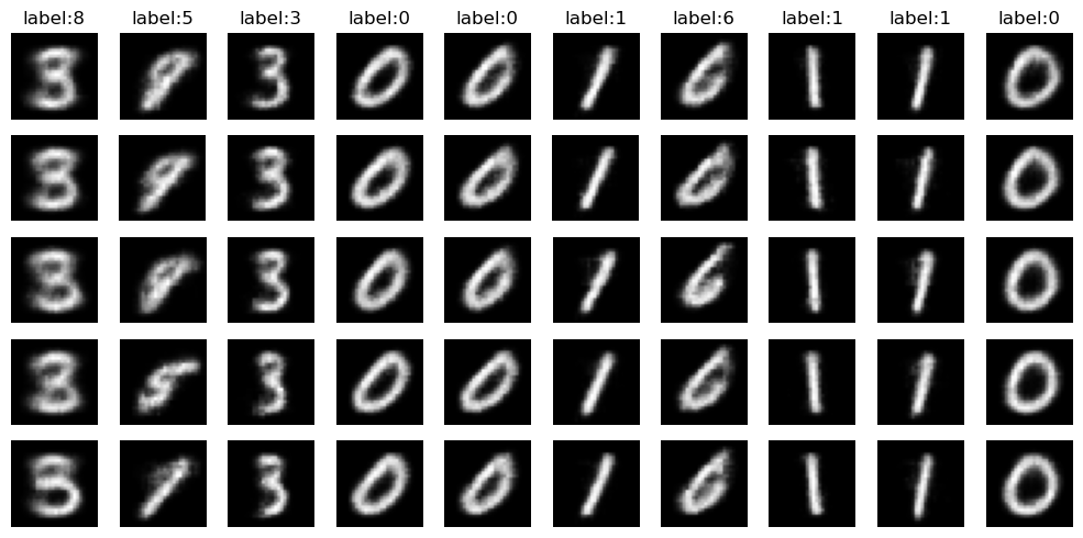
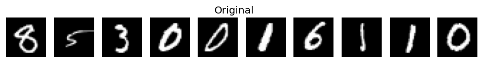
Above figure shows how the model reconstructions improve during the training. We showed the model’s reconstructions on 10 different images from the validation set. Reconstructions are obtained after every 10 epochs with the first row at the start of the training and last row showing the model’s outputs at the last epoch. They are plotted along with the original images for comparison.
Latent space
Latent space is an intermediate representation of the data compressed by the encoder. Think of it as a vector in an \(n\)-dimensional space where \(n\) is usually smaller than the actual data dimensions. Latent space is supposed to embed all the information of the input and should be sufficient to describe the data.
Here’s the definition of the latent space according to ChatGPT:
In machine learning, a latent space refers to a lower-dimensional representation of data that captures meaningful and useful information. It’s a concept commonly used in various techniques such as autoencoders, generative adversarial networks (GANs), and other dimensionality reduction methods.
For the purpose of this post and to keep things simple, we will keep the latent space dimension of our autoencoder model to be 2 so that we can visualize the encoded images by plotting the embeddings. The python code for creating the latent space is as follows:
example_ds = torch.utils.data.Subset(valid_data, range(5000))
latent_space = []
labels = []
for i in range(len(example_ds)):
	image, label = example_ds[i]
	model.eval()
	model = model.to("cpu")
	image = image[None, :, :, :]
	encoder_out, _ = model(image)
	encoder_out = encoder_out.detach().cpu().numpy().squeeze()
	latent_space.append(encoder_out)
	labels.append(label)
latent_space = np.array(latent_space)
The latent space for the random subset of 5000 validation set images is plotted in the following figure:
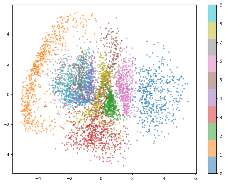
From the structure of the latent space above, it is clear that the model was able to find some pattern in the images and it tried grouping similar looking images together even though it had never seen the image labels.
Generating new images
In principle, once the model is trained, we can generate new images by just randomly sampling the latent space for some coordinates and pass them through the decoder. The decoder should then generate the new images. This can be easily implemented like so:
mins, maxs = np.min(latent_space, axis=0), np.max(latent_space, axis=0)
recon_examples = np.random.uniform(mins, maxs, size=(18, 2))
recon_examples_tensor = torch.tensor(recon_examples, dtype=torch.float32)
reconstructions = model.decoder(recon_examples_tensor).detach().cpu().numpy()
Problem with autoencoders
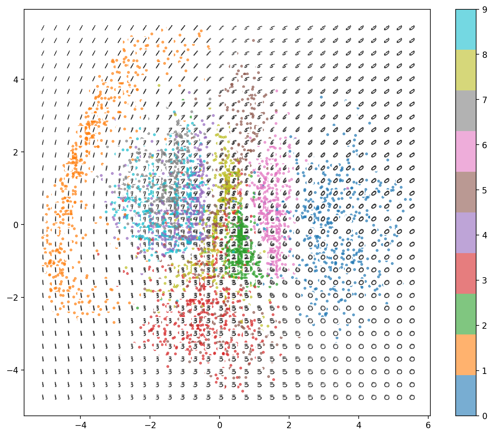
While generating the images by the method described in the previous section should work in theory, there are some serious issues with autoencoders. To understand it better, we can check the reconstructions obtained from the sampling of the points from the domain ranging from min to max of the latent space overlaid on the latent space like in the following image:
-
Some classes are concentrated in a much smaller area than the others. This will make a consistent sampling for all classes difficult because we will most likely to sample the classes which spanned larger area in the latent space
-
There are empty spaces between any two classes. Because of this if we randomly sample a point which lands in that empty space (specifically in the empty space between two classes), the model has no reason to choose one class over the other and the generated output will be non-recognizable
-
The distribution of the class examples in the latent space is not known and because of this autoencoders are not well suited for generating new images beyond reconstructing the inputs
-
For our example, we chose the latent space dimensions to be 2. This added a hard restriction on the autoencoder since it has lesser number of dimensions to encode the input, and because of this it squashed the information of the input labels in tight clusters. These clusters have relatively smaller gaps between them. However, if we increase the dimensions of our latent space, the above restriction is lifted off and we start seeing huge gaps between the clusters. This makes it even more complicated for autoencoder to generate well-formed images. The following plot shows the latent space with dimension 3:
So in a nutshell, there are similarities between autoencoders and generative model – both take a latent vector \(z\) as input and generate an output in the same space as the input. One huge difference between them is, for generative models, the features (like mean, standard deviation, shape, etc.) of the underlying distribution of latent space vector \(z\) are known which is not the case for an autoencoder. If a random sample comes from a distribution with known properties, we could sample the new points in the latent space from that distribution and generate a new image corresponding to each random sample. We can add this capability to the autoencoder by generalizing it into a so-called variational autoencoder.
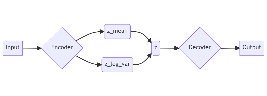
Variational Autoencoders (VAE)
In variational autoencoders, the encoder takes the input and it then maps it to the parameters of a standard normal distribution – the mean, \(\mu\) (z_mean), and the variance, \(\sigma^{2}\) (z_log_var). This is in contrast with the vanilla autoencoders where the encoder maps the input to a fixed point in the latent space. During training, apart from minimizing the reconstruction loss, the network also tries to match this \(\mu\) and \(\sigma^{2}\) to a standard normal distribution, \(\mathcal{N}(0, 1)\) (or more accurately, \(\mathcal{N}(0, \mathrm{I})\) where \(\mathrm{I}\) is an n-dimensional identity matrix). The vector \(z\) in the latent space is sampled from the distribution defined by parameters z_mean and z_log_var. After the VAE is trained, we can feed the random latent vectors to the decoer in order to generate new images.
Variance of a number is always positive and because of this we use logarithm of variance to make its range all real numbers. Standard deviation can be easily obtained from it by using the properties of standard logarithm:
\[\mathrm{z\_log\_var} = \log(\sigma^{2}) = 2 * \log(\sigma)\] \[\implies \sigma = e^{\mathrm{z\_log\_var} / 2}\]During training, the
z_log_varvariable will be converted to standard deviation (\(\sigma\)) using the reparameterization trick.
Reparameterization
To produce a random latent space vector \(z\) from the distribution defined by the \(\mu\) and \(\sigma\), we use the following equation:
\[z = \mu + \sigma * \epsilon\]where: \(\sigma = e^{log(\sigma^{2}) * 0.5}\;; \hspace{2 em}\epsilon \sim \mathcal{N}(0, \mathrm{I})\)
There are two ways in which the randomness to the latent space vector \(z\) can be inserted:
- Sampling directly the parameters
z_meanandz_log_varfrom a normal distribution. There is one big problem with this method which we will discuss in a bit - Sample the parameter \(\epsilon\) from a standard normal distribution, while keeping the parameters
z_meanandz_log_vartunable with backprogation. This is known as the reparameterization technique
Reparameterization allows us to break the above equation into deterministic and stochastic parts – all the randomness of the layer is packed within the parameter \(\epsilon\). We sample \(\epsilon\) from a normal distribution and then adjust the random vector to match to the correct mean and standard deviation. This process makes the backpropagation through the layer possible since the derivatives of the output with respect to input will be well-defined.
If instead, we try to compute \(z\) as \(\mu + \sigma\) with \(\mu\) and \(\sigma\) directly sampled from a normal distribution, the weights associated with the z_mean and z_log_var will be always changing. This will make the operation of calculating \(z\) to be non-deterministic and non-differentiable which means we can’t use the backpropagation to train the model. Moreover, without introducing any randomness we are removing the probabilistic nature of the latent space and hence the generative capabilities of the model. For each input \(x\) we will always get the same output \(y\) like in the case of vanilla autoencoders.
The objective function
For vanilla autoencoders, we only used the reconstruction loss term to optiize the weights during the training. This reconstruction loss tries to shuttle the whole training process in order to make the generated output look similar to the input images. In variational autoencoders, besides this reconstruction loss, we have an additional term called Kullback-Leibler (KL) divergence. This is an aymmetric metric used to measure how different is one probability distribution from a reference probability distribution.
As mentioned above, apart from minimizing the reconstruction loss, our network also tries to match the \(\mu\) and \(\sigma\) to a standard normal distribution during the training. KL divergence term is making sure of that – it penalizes the network when the \(\mu\) and \(\sigma\) start diverging from the standard normal distribution. Mathematically, it is described as –
\[D_{KL}(p(x)||q(x)) = \sum_{x \in X} p(x) \ln\frac{p(x)}{q(x)}\]where the \(p(x)\) is the baseline distribution, \(\mathcal{N}(0, \mathrm{I})\) in our case and \(q(x)\) is the sampling distribution which we want to match. Without going into the mathematical details, we can write the above equation in terms of the parameters of the two distributions:
\[D_{KL}(\mathcal{N}(\mu, \sigma) || \mathcal{N}(0, \mathrm{I})) = -\frac{1}{2} \sum(1 + \log(\sigma^{2})- \mu^{2} - \sigma^{2})\]where sum is over all the dimensions of the latent space.
VAE training
We built a convolutional VAE with a network architecture very similar to the vanilla autoencoder above. It consists of an encoder and decoder blocks connected to each other by the latent space vector. The network summary is as follows:
==========================================================================================
Layer (type:depth-idx)                   Output Shape              Param #
==========================================================================================
VariationalAutoencoder                   [32, 2]                   --
├─DownBlock: 1-1                         [32, 32, 14, 14]          --
│    └─Sequential: 2-1                   [32, 32, 14, 14]          --
│    │    └─Conv2d: 3-1                  [32, 32, 28, 28]          320
│    │    └─LeakyReLU: 3-2               [32, 32, 28, 28]          --
│    │    └─MaxPool2d: 3-3               [32, 32, 14, 14]          --
│    │    └─BatchNorm2d: 3-4             [32, 32, 14, 14]          64
├─DownBlock: 1-2                         [32, 64, 3, 3]            --
│    └─Sequential: 2-2                   [32, 64, 3, 3]            --
│    │    └─Conv2d: 3-5                  [32, 64, 7, 7]            18,496
│    │    └─LeakyReLU: 3-6               [32, 64, 7, 7]            --
│    │    └─MaxPool2d: 3-7               [32, 64, 3, 3]            --
│    │    └─BatchNorm2d: 3-8             [32, 64, 3, 3]            128
├─DownBlock: 1-3                         [32, 64, 1, 1]            --
│    └─Sequential: 2-3                   [32, 64, 1, 1]            --
│    │    └─Conv2d: 3-9                  [32, 64, 2, 2]            36,928
│    │    └─LeakyReLU: 3-10              [32, 64, 2, 2]            --
│    │    └─MaxPool2d: 3-11              [32, 64, 1, 1]            --
│    │    └─BatchNorm2d: 3-12            [32, 64, 1, 1]            128
├─Linear: 1-4                            [32, 2]                   130
├─Linear: 1-5                            [32, 2]                   130
├─Linear: 1-6                            [32, 64]                  192
├─UpBlock: 1-7                           [32, 64, 3, 3]            --
│    └─Sequential: 2-4                   [32, 64, 3, 3]            --
│    │    └─ConvTranspose2d: 3-13        [32, 64, 3, 3]            36,928
│    │    └─LeakyReLU: 3-14              [32, 64, 3, 3]            --
│    │    └─BatchNorm2d: 3-15            [32, 64, 3, 3]            128
├─UpBlock: 1-8                           [32, 32, 7, 7]            --
│    └─Sequential: 2-5                   [32, 32, 7, 7]            --
│    │    └─ConvTranspose2d: 3-16        [32, 32, 7, 7]            18,464
│    │    └─LeakyReLU: 3-17              [32, 32, 7, 7]            --
│    │    └─BatchNorm2d: 3-18            [32, 32, 7, 7]            64
├─UpBlock: 1-9                           [32, 16, 14, 14]          --
│    └─Sequential: 2-6                   [32, 16, 14, 14]          --
│    │    └─ConvTranspose2d: 3-19        [32, 16, 14, 14]          2,064
│    │    └─LeakyReLU: 3-20              [32, 16, 14, 14]          --
│    │    └─BatchNorm2d: 3-21            [32, 16, 14, 14]          32
├─ConvTranspose2d: 1-10                  [32, 1, 28, 28]           65
==========================================================================================
Total params: 114,261
Trainable params: 114,261
Non-trainable params: 0
Total mult-adds (M): 95.95
==========================================================================================
Input size (MB): 0.10
Forward/backward pass size (MB): 11.98
Params size (MB): 0.46
Estimated Total Size (MB): 12.54
==========================================================================================
The sample reconstructions from the model are obtained every 10 epochs and this is how they look during the course of training:
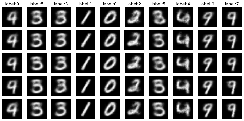
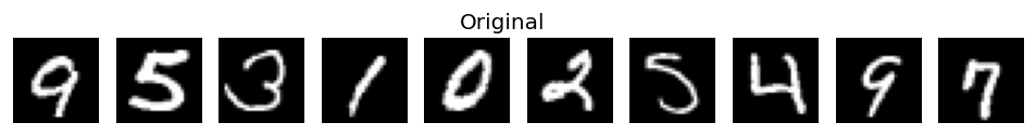
Like before, each row corresponds to the network’s reconstructions obtained on the same image every 10 epochs plotted along with the original image in the very end.
After training, we can plot the latent space embeddings and their corresponding normal CDF probabilities:
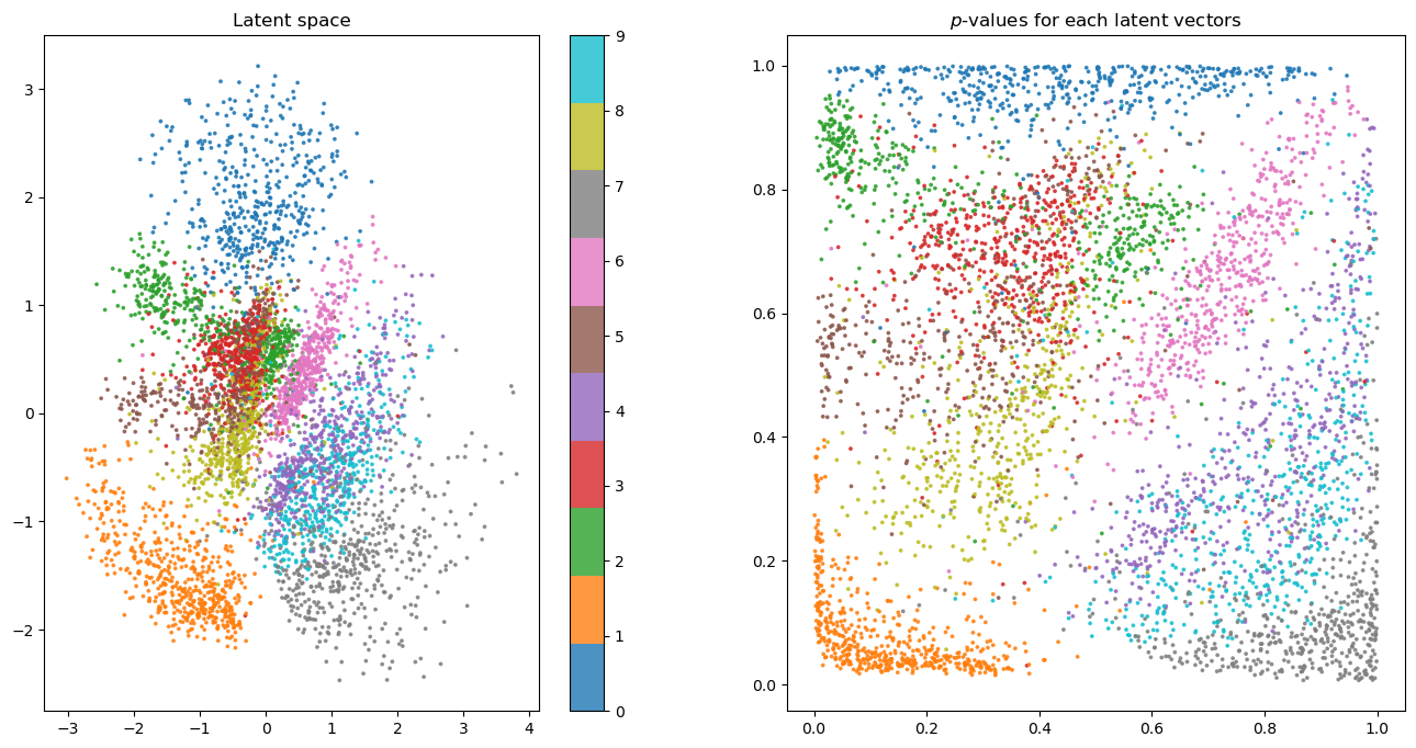
Plot on the left shows the latent space obtained from the variational autoencoder, it is very similar to the one obtained by the autoencoder and hence not very interesting. The righthand plot, on the other hand, shows the evenly spreaded latent space vectors when transformed into the normal distribution CDF probabilities. Recall that cumulative distribution function (CDF) tells us the probability that a random variable takes on a value less than or equal to some value. In our case, the random variable is the randomly sampled latent space vector and we can see that it captures almost all of the probability space with each class being represented almost equally.
References
- Generative Deep Learning, 2nd edition - David Foster (O’Reilly Media, Inc)
- Machine Learning with PyTorch and Scikit-learn - Sebastian Raschka, Yuxi Liu, Vahid Mirjalili, Dmytro Dzhulgakov (Packt Publishing)
- Auto-Encoding Variational Bayes - Diederik P Kingma, Max Welling
- Variational autoencoders - Jeremy Jordan